2 Description of the Problem

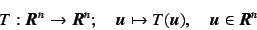
Let $T$ be a map described as follows:

$$T: \mbox{\boldmath$ R $}^n \rightarrow \mbox{\boldmath$ R $}... ... u $}), \quad \mbox{\boldmath$ u $}\in \mbox{\boldmath$ R $}^n$$ (1)

$T$ has explicit parameters $\lambda_1\in\mbox{\boldmath$\ R $}$ and $\lambda_2\in\mbox{\boldmath$\ R $}$ and $T$ is a $C^\infty$ map for these parameters. Then the fixed point $\mbox{\boldmath$\ u $}_0$ of Eq.(1) is given as

$$T(\mbox{\boldmath$ u $}_0) = \mbox{\boldmath$ u $}_0.$$ (2)

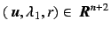
Assume now that this fixed point has at least a pair of complex conjugate multipliers described by:

$$\mu, \bar{\mu} = r e^{\pm i \theta}.$$ (3)

where, $r$ is the radius, $i$ is the imaginary unit and $\theta$ is the argument. If $\theta$ is specified, the location and the parameter value of the fixed point forms an isocline as the another parameter value changes.

Let $\mbox{\boldmath$\ J $}$ be the Jacobian matrix of $T$ around $\mbox{\boldmath$\ u $}_0$ and $\chi$ be the corresponding characteristic equation:

$$\chi = \mathop{\rm det}\nolimits [\mbox{\boldmath$ J $}- r e^{i\theta}] = \Re \chi + i \Im \chi = 0$$ (4)

where $\Re\chi$ and $\Im\chi$ show the real and imaginary part of the characteristic equation.

To calculate the location of the fixed point with specified argument, the following simultaneous equation should be solved with $(\mbox{\boldmath$\ u $}, \lambda_1, r)\in \mbox{\boldmath$\ R $}^{n+2}$ by using Newton's method:

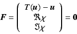$$\mbox{\boldmath$ F $} = \left( \begin{array}{c} T(\mbox{\bol... ... $}\\ \Re \chi \\ \Im \chi \end{array}\right ) = \mbox{\bf0}$$ (5)

Then the Jacobian matrix of the Eq.(5) is written as follows.

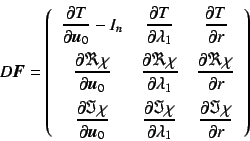$$D\mbox{\boldmath$ F $} = \left( \begin{array}{ccc} \displa... ...style \frac{\partial \Im\chi}{\partial r} \end{array}\right)$$ (6)

Note that all factors of the matrix in Eq.(6) are obtained by solving the variational equation of $T$. If $\theta$ is fixed as an appropriate value within $[0, \pi]$, the isocline is drawn in the parameter plane $\lambda_1$-$\lambda_2$ by plotting the solution $\lambda_1$ as the incremental parameter changes.

Now suppose that the parameter region in which the fixed point exists is already obtained. Firstly specifying $\theta=0$ or $\theta=\pi$, we obtain an isocline which splits the parameter region into two parts; the part has is a sink, the other has a stable node. Therefore this isocline can be regarded as a bifurcation curve. For any rational ratio with $\pi$ of $\theta$, the corresponding isocline shows instantaneous phase around the fixed point and it is deeply related to the NS bifurcation and existence of frequency entrainment regions. Along this isocline, the stability is indexed by $r$, i.e., within $0\le r < 1$, we have a stable sink, and $r = 0$ shows a super stable sink.